This is the fourth chapter of the DB engineering series. As a prerequisite ensure that you read the previous chapters.
Jump to other chapters:
- 01. Understanding database storage
- 02. Database Indexes
- 03. Understanding EXPLAIN & ANALYZE
- 04. Partitioning
- 05. Sharding
- 06. Transactional vs Analytical Databases
As more and more rows get added to the table, the database has to scan more pages and data. Queries are bound to become slower. Indexes will help to a great extent. But when dealing with an order of millions, one of the strategies to improve query performance is to partition the table.
Just like the name suggests, we split the large table into smaller tables. There are two types of partitions – horizontal partitioning and vertical partitioning.
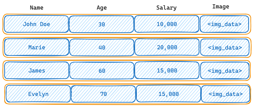
Consider the table below.

Vertical Partitioning
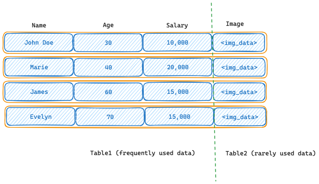
The application might be querying the name, age, and salary attributes frequently. If the image column is rarely used, we are unnecessarily increasing the scan time for queries.
One strategy of optimization is to partition the table vertically. We can move the image attribute to a different table.

The table2 can reside in a slower HDD while the frequently used table resides in a faster SSD. That way we are saving compute and storage resources. Do not confuse this approach with the normalization of the tables. Normalization of data is at a conceptual level, whereas vertical partitioning is done at a physical level. An already normalized table may be split again through vertical partitioning for performance gains and DB management.
Horizontal partitioning
Let’s say we split the table into 2 smaller tables – one which has all the data of people who are less than 50 years of age and another for people above 50 years of age.

Here we are partitioning the table based on the value of an attribute. By splitting the large table into smaller ones, especially when queries are made for age predicate (eg: SELECT * FROM people WHERE age < 30), the DB will have to only deal with the smaller table1.
Partition by
The are a few methods by which we can split the tables horizontally.
Range partitioning
Range partitioning is the most common type of partitioning. It is employed to separate a table into value ranges. For example, you could make a table with a year column and then divide it into partitions for each month. That way, we would be able to quickly fetch the data for a certain month.
List partitioning
List partitioning is used to divide a table into a list of known values. For example, you could create a table with a country column and then partition it into partitions for each country. This would allow you to quickly and easily access data for a specific country.
Hash partitioning
Hash partitioning distributes rows evenly across partitions using a hash function.
Hands-on
Alright, time to get our hands dirty.
Let’s drop the table people and recreate it with 20M rows.
DROP table people;
CREATE TABLE people (
  id serial PRIMARY KEY,
  name text,
  age int,
  salary int
);
INSERT INTO people (name, age, salary)
SELECT
substring('ABCDEFGHIJKLMNOPQRSTUVWXYZabcdefghijklmnopqrstuvwxyz0123456789', (random() * 62 + 1)::int, 5),
random() * 100 + 18,
random() * 100000 + 10000
FROM generate_series(1, 20000000);
Let’s check how our original query to fetch all people who are 40 years old performs.
QUERY I
                                                           learning_test=> explain analyze select * from people where age = 40;
                                                           QUERY PLAN
--------------------------------------------------------------------------------------------------------------------------------
 Gather  (cost=1000.00..249146.95 rows=173999 width=17) (actual time=13.921..3465.305 rows=198712 loops=1)
   Workers Planned: 2
   Workers Launched: 2
   ->  Parallel Seq Scan on people  (cost=0.00..230747.05 rows=72500 width=17) (actual time=9.175..3402.664 rows=66237 loops=3)
         Filter: (age = 40)
         Rows Removed by Filter: 6600429
 Planning Time: 10.044 ms
 JIT:
   Functions: 6
   Options: Inlining false, Optimization false, Expressions true, Deforming true
   Timing: Generation 0.571 ms, Inlining 0.000 ms, Optimization 0.605 ms, Emission 26.737 ms, Total 27.914 ms
 Execution Time: 3522.797 ms
(12 rows)
Yikes! That took approximately 3.5 seconds to do a sequential scan of the whole table.
Let’s create a new people_partitioned table identical to people table. In addition, we will partition the table based on the age.
learning_test=> CREATE TABLE people_partitioned (
  id serial PRIMARY KEY,
  name text,
  age int,
  salary int
) PARTITION BY RANGE(age);
ERROR:  unique constraint on partitioned table must include all partitioning columns
DETAIL:  PRIMARY KEY constraint on table "people_partitioned" lacks column "age" which is part of the partition key.
Oops! The error means that you cannot create a unique constraint on a partitioned table unless the constraint includes all of the partitioning columns. In this case, the table is partitioned by the age column, but the PRIMARY KEY constraint only includes the id column. To fix this error, let’s remove the PRIMARY KEY constraint.
learning_test=> CREATE TABLE people_partitioned (
  id serial,
  name text,
  age int,
  salary int
) PARTITION BY RANGE(age);
CREATE TABLE
Now let’s create partitions for the main table. We will split the table by age into 3 segments. 0-40, 40-80, and 80 to 120. We will create 3 tables just “like” the main table.
learning_test=> CREATE TABLE people_age0040 (LIKE people_partitioned);
CREATE TABLE
learning_test=> CREATE TABLE people_age4080 (LIKE people_partitioned);
CREATE TABLE
learning_test=> CREATE TABLE people_age80120 (LIKE people_partitioned);
CREATE TABLE
The next step is to attach the partitions to the main table. We will also specify the values. Note the FOR VALUES FROM X TO Y clause.
learning_test=> ALTER TABLE people_partitioned ATTACH PARTITION people_age0040 FOR VALUES FROM (0) TO (40);
ALTER TABLE
learning_test=> ALTER TABLE people_partitioned ATTACH PARTITION people_age4080 FOR VALUES FROM (40) TO (80);
ALTER TABLE
learning_test=> ALTER TABLE people_partitioned ATTACH PARTITION people_age80120 FOR VALUES FROM (80) TO (120);
ALTER TABLE
Alright, now we have created a table partitioned by age. A little bit of terminology.
- The
people_partitionedtable is avirtualtable. The data resides in 3 other partitions. - The partitions are segmented based on age. Each partition stores a subset of the data as defined by its
partition bounds. - The
paritioning methodwe used inrangepartitioning. - The partitions are created based on the values of
agealso known as thepartition key. - You can ATTACH and DETACH partitions by ALTERing the original table. DETACHing and DROPing a partition is one way of removing unwanted data (for example drop logs from last year).
We will now copy all the data from our original people table into people_partitioned table.
learning_test=> INSERT INTO people_partitioned SELECT * FROM people;Now, EXPLAINing the SELECT of the same results from people_partitioned table will give us the following output.
QUERY II
                                                                       learning_test=> explain analyze select * from people_partitioned where age = 40;

QUERY PLAN
---------------------------------------------------------------------------------------------------------------------------------------------------------
 Gather  (cost=1000.00..112892.64 rows=195987 width=17) (actual time=4.977..1073.677 rows=198712 loops=1)
   Workers Planned: 2
   Workers Launched: 2
   ->  Parallel Seq Scan on people_age4080 people_partitioned  (cost=0.00..92293.94 rows=81661 width=17) (actual time=8.873..883.694 rows=66237 loops=3)
         Filter: (age = 40)
         Rows Removed by Filter: 2600286
 Planning Time: 3.732 ms
 JIT:
   Functions: 6
   Options: Inlining false, Optimization false, Expressions true, Deforming true
   Timing: Generation 0.523 ms, Inlining 0.000 ms, Optimization 0.553 ms, Emission 25.929 ms, Total 27.006 ms
 Execution Time: 1101.750 ms
(12 rows)
A few things to note in the above output (compare Query I and Query II).
- The execution time is lower (1101ms vs 3522ms).
- The cost of the query is lower (112892 vs 249146).
- The sequential scan of Query II is performed on
people_age4080 people_partitionedtable, a smaller subset of the original data.
How can we optimize this further? Obviously by creating an index.
learning_test=> CREATE INDEX idx_age_people_partitioned ON people_partitioned(age);
learning_test=> CREATE INDEX idx_age_people ON people(age);
Now that indexes are created for both original and partitioned table, let’s compare the queries.
Query III
Query the original table now with an index.
learning_test=> explain analyze select * from people where age = 40;
                                                                 QUERY PLAN
--------------------------------------------------------------------------------------------------------------------------------------------
 Gather  (cost=2940.94..224952.62 rows=174000 width=17) (actual time=98.693..1567.347 rows=198712 loops=1)
   Workers Planned: 2
   Workers Launched: 2
   ->  Parallel Bitmap Heap Scan on people  (cost=1940.94..206552.62 rows=72500 width=17) (actual time=45.270..1449.138 rows=66237 loops=3)
         Recheck Cond: (age = 40)
         Rows Removed by Index Recheck: 3433617
         Heap Blocks: exact=11698 lossy=22916
         ->  Bitmap Index Scan on idx_age_people  (cost=0.00..1897.44 rows=174000 width=0) (actual time=74.074..74.075 rows=198712 loops=1)
               Index Cond: (age = 40)
 Planning Time: 0.085 ms
 JIT:
   Functions: 6
   Options: Inlining false, Optimization false, Expressions true, Deforming true
   Timing: Generation 0.627 ms, Inlining 0.000 ms, Optimization 0.639 ms, Emission 14.759 ms, Total 16.025 ms
 Execution Time: 1580.827 ms
(15 rows)
Query IV
Here we query the partitioned table now with an index added on top of the partitions.
learning_test=> explain analyze select * from people_partitioned where age = 40;
                                                                       QUERY PLAN
--------------------------------------------------------------------------------------------------------------------------------------------------------
 Bitmap Heap Scan on people_age4080 people_partitioned  (cost=2183.35..55263.21 rows=195989 width=17) (actual time=26.506..250.948 rows=198712 loops=1)
   Recheck Cond: (age = 40)
   Heap Blocks: exact=49630
   ->  Bitmap Index Scan on people_age4080_age_idx1  (cost=0.00..2134.35 rows=195989 width=0) (actual time=14.550..14.551 rows=198712 loops=1)
         Index Cond: (age = 40)
 Planning Time: 0.142 ms
 Execution Time: 261.585 ms
(7 rows)
Learnings from Query III and Query IV
- An index added on top of the partition looks more performant.
- Adding an index to
people_partitionedtable automatically adds indexes for partitions. - Each of the separate partitions has its own index.
- The cost of the query with partition+index is significantly lesser.
Additional notes
Query performance can be increased by partitioning a large table. However, your mileage may vary depending on the table size and the type of query. When the table size exceeds the size of the memory of the server, you will start seeing improvements after partitioning.
DELETE queries on large tables will require VACUUM to free up the disk space. In the case of partitioned tables, DETACHing and DROPping an unwanted partition will immediately free up the disk space. Partitioning of tables can thus be used for table maintenance.
In partitioning, the smaller tables reside in the same database server. What if we want to split the data to be handled by multiple database servers? Read about sharding here.
